Derivation of Decimation-in-Time Fast Fourier Transform

I chose to implement the decimation-in-time (DIT) form of a FFT not because I thought it would result in an efficient implementation but rather because the algorithm seemed conceptually simpler. I have favored simplicity over efficiency since this is my first verilog design.

The definition of a discrete fourier transform (DFT) is

\begin{equation*} X_k = \sum_{n=0}^{N-1}{x_n e^{-2 \pi i k n/N}} \end{equation*}

where \(x_n\) is a sequence of length \(N\) and \(X_k\) is the fourier transform of this sequence.

The most common FFT algorithm is the Cooley-Tukey FFT algorithm which takes advantage of the fact that a discrete fourier transform (DFT) can be expressed in terms of a combination of two smaller DFTs.

Let \(e_n\) be the even components of \(x_n\) (\(e_n = x_{2n}\)).

Let \(o_n\) be the odd components of \(x_n\) (\(o_n = x_{2n+1}\)).

Let \(E_k\) and \(O_k\) be their DFTs.

\begin{equation*} \begin{aligned} X_k & = \sum_{n=0}^{N-1}{x_n e^{-2 \pi i k n/N}} \\ & = \sum_{n=0}^{N/2-1}{x_{2n} e^{-4 \pi i k n/N}} + \sum_{n=0}^{N/2-1}{x_{2n+1} e^{-2 \pi i k (2n+1)/N}} \\ & = \sum_{n=0}^{N/2-1}{e_n e^{-2 \pi i k n/(N/2)}} + e^{-2 \pi i k/N}\sum_{n=0}^{N/2-1}{o_n e^{-2 \pi i k /(N/2)}} \\ & = E_k + e^{-2 \pi i k/N} O_k \end{aligned} \end{equation*}

Since DFTs wrap around, \(E_k = E_{k-N/2}\), and \(e^{ix} = -e^{i(x+\pi)}\), we can write \(X_k\) as:

\begin{equation*} \begin{aligned} X_k & = E_k + e^{-2 \pi i k/N} O_k \\ X_{k+N/2} & = E_k - e^{-2 \pi i k/N} O_k \end{aligned} \end{equation*}

Equations 1 and 2

so that we only need to consider \(0 < k \le N/2\) to generate all of \(X_k\).

Using these equations the DFT is calculated in a series of stages where in each stage we calculate a new set of N complex numbers from the N complex number of the previous stage.

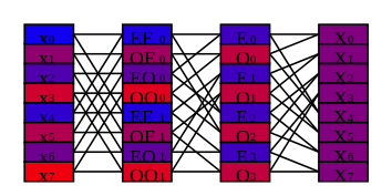
Figure 1: Schematic of DFT of size 8.

Figure 1 shows a schematic of the calculation of a DFT of size 8. The column of rectanges on the left represent \(x_n\), the input data to the DFT (the zeroth stage). The column of rectangles on the right represent \(X_k\), the output of the DFT (the third stage). In between are two intermediate stages. The data in the second stage is labelled with \(E_k\) and \(O_k\) so that we can see how to apply equations 1 and 2 to calculate the third stage from the second. The data in the first stage is labelled with \({EE}_k\), \({OE}_k\), \({EO}_k\), and \({OO}_k\), where \({OE}_k\) is the fourier transform of \({oe}_n\) which is the even components of \(o_n\), the odd components of \(x_n\). We can calculate \(E_k\), using equations 1 and 2, from \({EE}_k\) and \({EO}_k\), and similarly we calculate \(O_k\) from \({OE}_k\) and \({OO}_k\). The lines in Figure 1 show the dataflow from one stage to the next.

In general, stage \(s\) is an interleaving of \(S=N/2^s\) transforms of length \(M=N/S\). Let \(P_{s,i}\) be component \(i\) of stage \(s\). Let \(X_{s,j,k}\) be component \(k\) of transform \(j\) in stage \(s\). So in Figure 1 \(E_3\) is component 6 (we index from 0) of stage 2, \(P_{2, 6}\), and is also component 3 of transform 0 of stage 2, \(X_{2, 0, 3}\).

\begin{equation*} X_{s,j,k} = P_{s,kS+j} \end{equation*}

The DFT \(X_{s,j,k}\) (\(k\) is position in the DFT) was generated by combining two DFTs from the previous stage, \(X_{s-1,j,k}\) and \(X_{s-1,j+S,k}\). We then have,

\begin{equation*} \begin{aligned} X_{s,j,k} & = X_{s-1,j,k} + e^{-2 \pi i kS/N} X_{s-1,j+S,k} \\ P_{s,kS+j} & = P_{s-1,2kS+j} + e^{-2 \pi i kS/N} P_{s-1,2kS+S+j} \\ P_{s,kS+j} & = P_{s-1,2kS+j} + T_{kS} P_{s-1,2kS+S+j} \end{aligned} \end{equation*}

Equation 3

where \(T_{n} = e^{-2 \pi i n/N}\).

And similarly for the second half of P we have,

\begin{equation*} P_{s,kS+j+N/2} = P_{s-1,2kS+j} - T_{kS} P_{s-1,2kS+S+j} \end{equation*}

Equation 4

This completes the derivation of the algorithm and in the next section we'll describe the verilog implementation.

Next: Implementation of FFT algorithm.